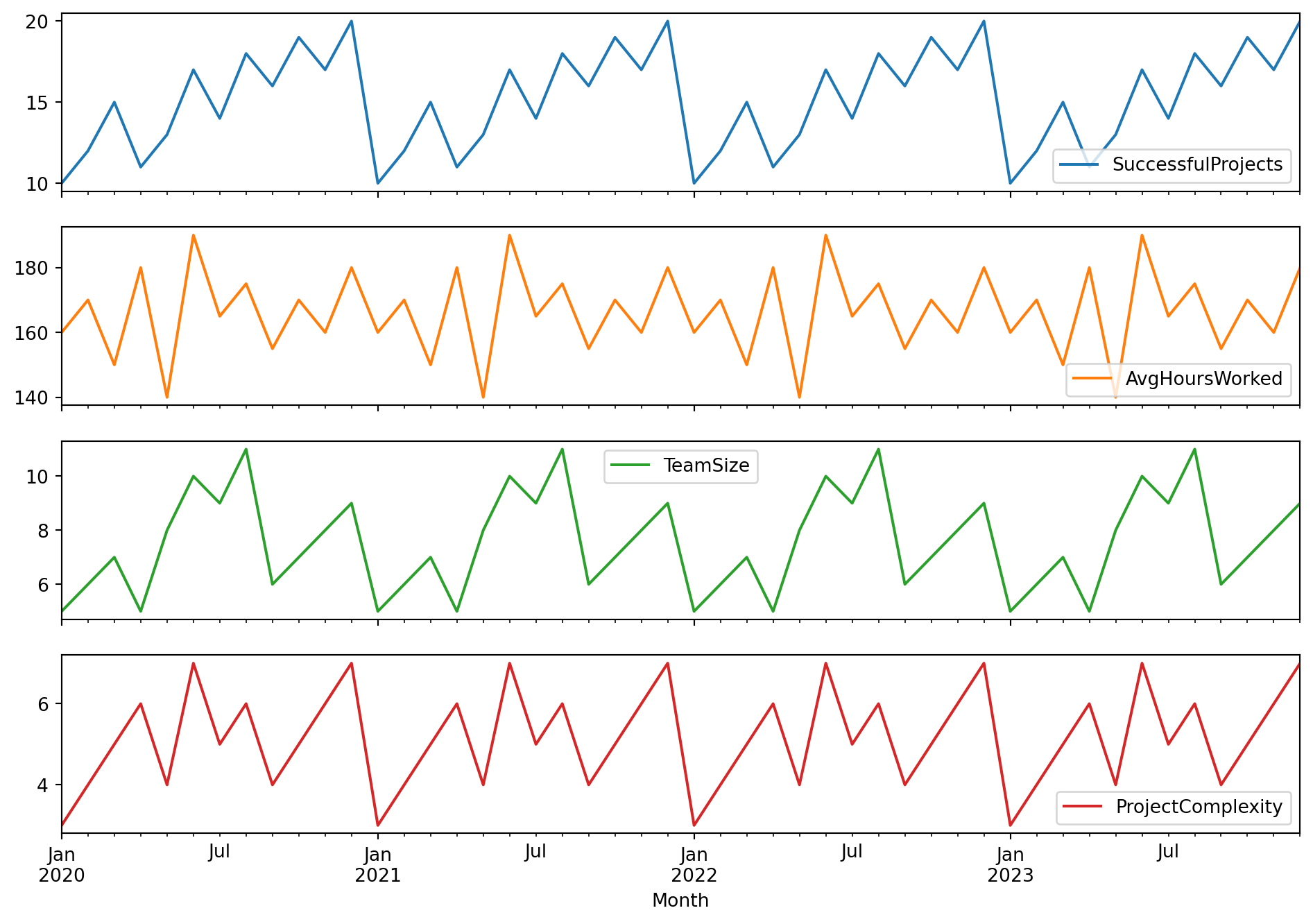
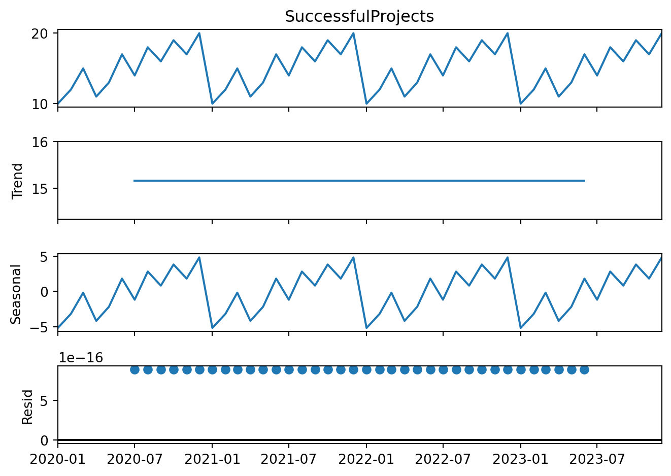
Time Series Example

Example of Dummy Data

Code

import pandas as pd
import matplotlib.pyplot as plt
from statsmodels.tsa.seasonal import seasonal_decompose
from statsmodels.tsa.stattools import adfuller
import warnings

# Dummy dataset
data = {
    'Month': pd.date_range(start='2020-01-01', end='2023-12-01', freq='MS'),
    'SuccessfulProjects': [10, 12, 15, 11, 13, 17, 14, 18, 16, 19, 17, 20] * 4,
    'AvgHoursWorked': [160, 170, 150, 180, 140, 190, 165, 175, 155, 170, 160, 180] * 4,
    'TeamSize': [5, 6, 7, 5, 8, 10, 9, 11, 6, 7, 8, 9] * 4,
    'ProjectComplexity': [3, 4, 5, 6, 4, 7, 5, 6, 4, 5, 6, 7] * 4
}
df = pd.DataFrame(data)
df.head()

	Month	SuccessfulProjects	AvgHoursWorked	TeamSize	ProjectComplexity
0	2020-01-01	10	160	5	3
1	2020-02-01	12	170	6	4
2	2020-03-01	15	150	7	5
3	2020-04-01	11	180	5	6
4	2020-05-01	13	140	8	4

Exploratory Data Analysis

Code

df.set_index('Month', inplace=True)

# Plotting the data
df.plot(figsize=(12, 8), subplots=True)
plt.show()

# Decompose the time series (for successful projects only, for simplicity)
decomposition = seasonal_decompose(df['SuccessfulProjects'], model='additive')
fig = decomposition.plot()
plt.show()

Model Building

Code

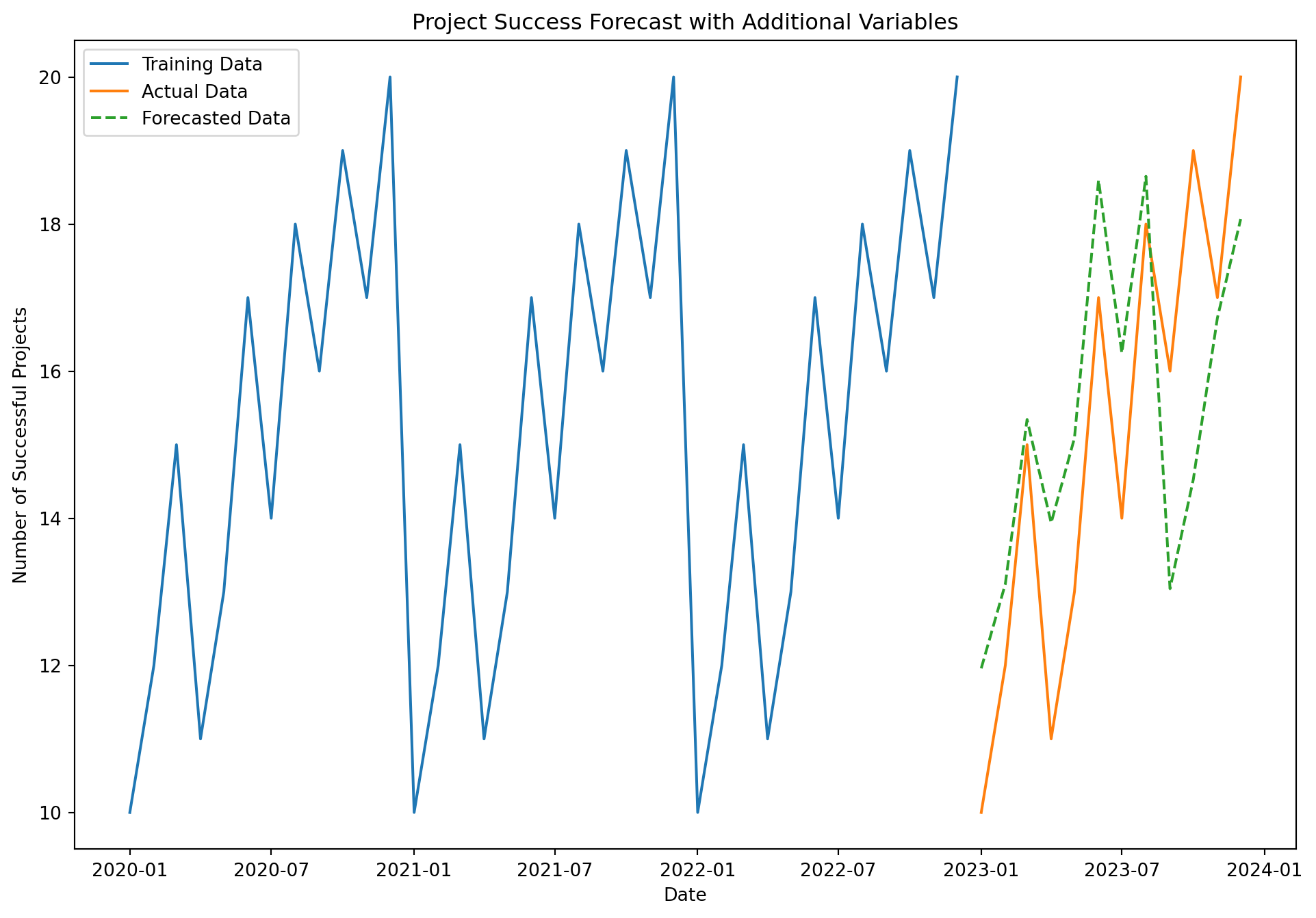
from statsmodels.tsa.statespace.sarimax import SARIMAX

# Suppress specific warnings
warnings.filterwarnings("ignore", message="no frequency information was provided")

# Splitting the data into training and testing sets
train = df[:'2022']
test = df['2023':]

# Building the ARIMAX model with adjustments to improve convergence
model = SARIMAX(
    train['SuccessfulProjects'], 
    exog=train[['AvgHoursWorked', 'TeamSize', 'ProjectComplexity']], 
    order=(1, 1, 1),
    enforce_stationarity=False,
    enforce_invertibility=False
)
model_fit = model.fit(disp=False, maxiter=500, method='nm')

# Summary of the model
print(model_fit.summary())

# Forecasting
forecast = model_fit.get_forecast(steps=len(test), exog=test[['AvgHoursWorked', 'TeamSize', 'ProjectComplexity']])
forecast_df = test.copy()
forecast_df['Forecast'] = forecast.predicted_mean

# Plotting the actual vs forecasted values
plt.figure(figsize=(12, 8))
plt.plot(train['SuccessfulProjects'], label='Training Data')
plt.plot(test['SuccessfulProjects'], label='Actual Data')
plt.plot(forecast_df['Forecast'], label='Forecasted Data', linestyle='--')
plt.title('Project Success Forecast with Additional Variables')
plt.xlabel('Date')
plt.ylabel('Number of Successful Projects')
plt.legend()
plt.show()

                               SARIMAX Results                                
==============================================================================
Dep. Variable:     SuccessfulProjects   No. Observations:                   36
Model:               SARIMAX(1, 1, 1)   Log Likelihood                 -69.563
Date:                Wed, 10 Jul 2024   AIC                            151.127
Time:                        15:09:26   BIC                            160.106
Sample:                    01-01-2020   HQIC                           154.148
                         - 12-01-2022                                         
Covariance Type:                  opg                                         
=====================================================================================
                        coef    std err          z      P>|z|      [0.025      0.975]
-------------------------------------------------------------------------------------
AvgHoursWorked       -0.0284      0.041     -0.690      0.490      -0.109       0.052
TeamSize              0.7813      0.249      3.139      0.002       0.293       1.269
ProjectComplexity     1.1319      0.612      1.848      0.065      -0.068       2.332
ar.L1                 0.5053      0.257      1.967      0.049       0.002       1.009
ma.L1                -1.0000   1458.798     -0.001      0.999   -2860.192    2858.191
sigma2                3.6376   5306.701      0.001      0.999   -1.04e+04    1.04e+04
===================================================================================
Ljung-Box (L1) (Q):                   0.03   Jarque-Bera (JB):                 1.79
Prob(Q):                              0.86   Prob(JB):                         0.41
Heteroskedasticity (H):               0.91   Skew:                             0.31
Prob(H) (two-sided):                  0.88   Kurtosis:                         2.05
===================================================================================

Warnings:
[1] Covariance matrix calculated using the outer product of gradients (complex-step).

Model Evaluation

Code

from sklearn.metrics import mean_absolute_error, mean_squared_error

# Evaluation metrics
mae = mean_absolute_error(test['SuccessfulProjects'], forecast.predicted_mean)
mse = mean_squared_error(test['SuccessfulProjects'], forecast.predicted_mean)
print(f'Mean Absolute Error: {mae}')
print(f'Mean Squared Error: {mse}')

Mean Absolute Error: 1.8805247500041948
Mean Squared Error: 4.89588917787364